Learning on an analytic base

01 / Let the base explain the geometry

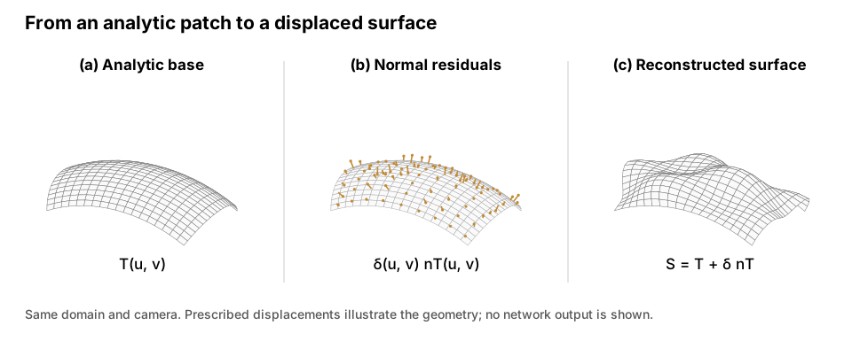
A local neural surface model can spend its capacity describing geometry that is already available analytically. Neural Toroidal Patch starts from an osculating torus and asks a small network to predict the remaining displacement along the torus normal.

S(u, v) = T(u, v) + δ_θ(u, v, z_i) n_T(u, v)

Here T gives the analytic base point, nT is its unit normal, and δθ is a scalar residual predicted from local coordinates and a patch code zi. The base, pose and domain turn local coordinates into a geometric surface; the network adds detail.

This decomposition changes what the learning problem asks the network to explain. The network does not need to discover the patch position, orientation and complete low-frequency geometry from scratch. Those are supplied by the analytic construction. Its output is one signed distance along a known normal direction, so a local surface point is obtained by combining geometry and prediction.

The sign of the residual chooses which side of the base contains the reconstructed point. A zero residual leaves the point on the torus. This makes the representation easy to inspect geometrically, but it also imposes a modeling assumption: the desired local surface should be expressible as a suitable normal displacement of the chosen base.

* * *

02 / Inspect a normal displacement

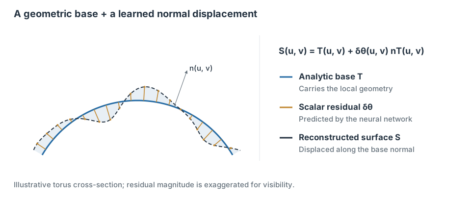
Analytic toroidal patch, prescribed normal residuals, and displaced surface — Three views of the same patch domain. Gold segments are signed displacements along the analytic unit normal. This computed example illustrates the representation; the residual field is prescribed, not predicted by a trained model.

Normal residual added to an analytic base

Illustrative cross-section. Adjusting the scale changes a prescribed displacement; it does not train a network or report reconstruction accuracy.

Base pointChoose a point on the blue analytic cross-section.
Scalar residualMove by a signed amount along its normal. Gold segments connect the base to the reconstructed curve.
Reconstructed pointThe dashed curve contains the displaced points. At zero residual it coincides with the base.

* * *

03 / Share the network, keep a code for each patch

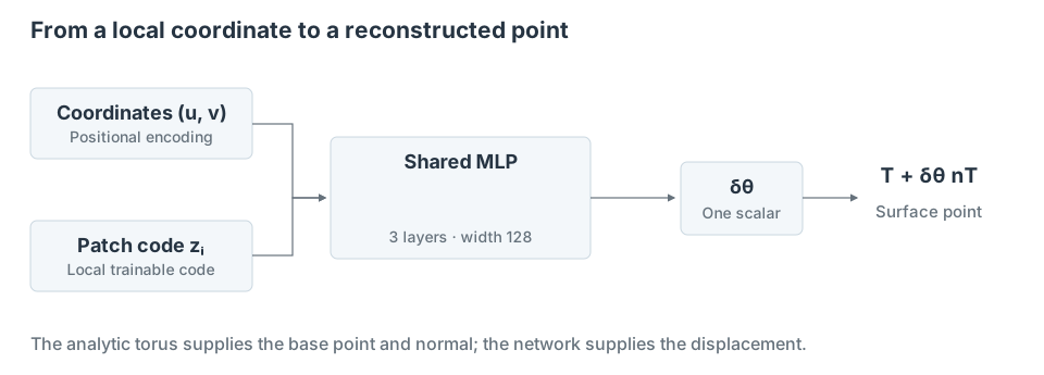
The manuscript uses a plain three-layer, width-128 MLP. The torus supplies geometric structure outside the network; per-patch codes supply local adaptability.

Under the fixed patch decomposition used in the study, the tested architectural additions did not improve on the plain small MLP. The comparison therefore asks not only how to make a network larger, but which geometric information should be provided before learning starts.

The transfer experiment shares a network across training shapes and adapts held-out shapes by optimizing their patch codes. This keeps the learned residual model fixed during adaptation while giving each new patch local degrees of freedom.

The per-patch code and the shared network serve different purposes. The code identifies local variation that cannot be inferred from the coordinates alone. The shared weights learn a common way to turn coordinates and codes into residuals. Without patch-specific information, identical parameter coordinates on different patches would not be sufficient to specify their different residual fields.

The transfer experiment tests whether the shared weights contain reusable information. When only codes are optimized for held-out shapes, the network itself cannot change to fit each new object. Comparing this adaptation with a randomly initialized frozen network helps distinguish learned transfer from the flexibility of the local codes alone.

* * *

04 / What the comparisons support

The strongest distinction in the reported smooth-mesh experiments is whether a local analytic base is present. An osculating torus, an osculating paraboloid and a tangent plane achieve comparable accuracy under the controlled setup, while the capacity-matched base-free model is substantially worse.

The base also helps when supervision becomes sparse. These comparisons support treating local geometry as a useful prior, while leaving room to choose a base according to the shape and computational task.

A controlled base comparison needs a common patch decomposition: otherwise, a method could appear better because it received easier or smaller regions. The study holds that decomposition and the training protocol fixed while changing the base or network. This makes the comparison informative about the contribution of the analytic prior within the tested setup.

The experiments also distinguish error at supervised vertices from behavior between them. Matching training samples does not by itself guarantee a good continuous surface. Evaluating points between vertices checks whether the representation interpolates the geometry sensibly, while sparse-supervision experiments test how strongly it depends on dense samples.

What this does not establishThe results concern the studied smooth meshes and fixed decompositions. A scalar normal displacement restricts the local surface family, and independent patches do not automatically provide global continuity. The study does not establish that the torus is universally the best base for sharp features or CAD-dominated models.

* * *

Research manuscript

Jinyoung Choi & Youngjin Park.
Neural Toroidal Patch: On Smooth Meshes, the Presence of a Local Analytic Base Matters More Than Its Form or the Network Architecture.Research manuscript · This overview summarizes its controlled comparisons.

For the underlying analytic patch construction, see toroidal patches and spatial queries.